Making the foundations of the Guassian Distribution more intuitive

–Warning - typos ahead—-

Perhaps the one topic in all statistics that is as prevalent as it is shrouded in mystery. Your professors and seniors failed to explain it and great textbooks introduce by pulling it out of a magic hat. In this blog we will show why the Guassian has some very natural properties and why it is critical is describing noisy or random phonemon and observations like like the one it was discovered to understand(access? better word). We want to understand why errors are considered normally distributed in linear regression and other ML algorithms and why the mean is used as a representiative number in many cases. I hope that the connection of random errors to the normal distribution blows your mind!

Here we will take part in function finding. Narrowing down the possible functions via figuring out properties that our function must obey. Perhaps an easier way to know the prevelance of the Gaussian is to identify some key properties and once we see a situation where we must have those, we can guess its the Guassian. I guarentee you after this( and some of your own thought) you will walk away finding the foundations of the Guassian more intuitive

First let’s consider X follows a Uniform distribution from 0 to 1 or $X\sim U(a,b)$ $X\sim U(0,1)$

We know the mean or the expected value of this distribution is equal to $1/2$. But what does $1/2$ really represent? If we were to sample a few or even a lot of points then there is guarentee that their average would be our theoretical expercted value. The defination of the expected value says that if we were to sample $N$ points, each $x_i$, then in the limit as $N$ tends to infinity the average would converge to the expected value. Stated succinctly as : $lim_{N\mapsto \infty} \frac{\sum_i^Nx_i}{N}\mapsto 1/2$

Let’s play around with this. Every point in X can be represented as how much it deviates from the excepted value as $1/2 + d_i$. Points to the left have a negative deviation and the right have posistive ones. E.g)

0.6 = 0.5 + 0.1

0.4 = 0.5 - 0.1

As the uniform is symteric around its mean you can image what the distribution of deviations would look like. The plot of the distribution of deviations $d_i$ is:

We see some nice properties of this distribution:

1) The distribution is symettric about 0

2)I am just as likely to get +0.1 as -0.1 or -0.2 as +0.2. For every positive value there is a equal negative value that occurs with the same probability

3)If I were to sum up all the points in this distribution, I would get 0 (again due to the symettry around 0)

Let’s consider the equally spread and finite number of points $0.1,0.2,0.3,0.4,0.5,0.6,0.7,0.8,0.9,1$ from X for demonstration. What if I were to change these to our alternate representation and sum them? Let’s see what happens: $\sum x_i = \sum 0.5 - d_i$ $\sum x_i = (0.5-0.4) + (0.5-0.3) + (0.5-0.2) + (0.5-0.1) + (0.5-0) + (0.5+0.1) + (0.5+0.2)+ (0.5+0.3) + (0.5+0.4)$ $\sum x_i = 10*0.5 = 5$

With our transformation $x_i=1/2+d_i$ you can see that every $d_i$ above 0.5 would cancel with every below. You can imagine this same result if I were to to it for the entire distribution and not just our discrete points. All the deviations would cancel each other out and I would be left with N times 1/2. (Keep in mind here we just summing the entire distribution and sampling and summing).

From this we get our first defination of the mean: the mean is the number around which the deviations cancel each other out when summed.

We will see that this holds for non-symettric distirbutions as well. This is useful because if my deviations were some random errors, then on summing them they would disappear. But more about that later.

The above is conveyed in the mean formula as well: (we will be seeing this formulae from many different angles in this blog)

\[\frac{\sum x_i}{N}=\bar{x}\] \[\sum x_i=N\bar{x}\]

This says something very similar about not needing to know every value to get the sum, although abit idealistically. We got the same thing when we summed our 10 points above. In our case we did:

$\sum x_i = \sum (\bar{x} + d_i) = \sum \bar{x} +\sum d_i $

And then using $\sum d_i = 0$

$\sum \bar{x} +\sum d_i = \sum \bar{x} +0 = N\bar{x}$

$\sum d_i$ = 0 is visually appreant in our case of summing the whole distribution, but in random sampling all deviations may not perfectly cancel out. We would expect most of them to, using observation 2 above, but it won’t be perfect. The idea that remains is that given a lot of obervations we would very well approximate $\sum x_i$ by $N\bar{x}$ as we would expect all the positive and negative deviations to cancel each other out. This idea of thinking about the deviations will be useful later on.

Simulating random points from the uniform gives me:

a=np.random.uniform(size=10)

array([0.80714911, 0.34312811, 0.51680355, 0.73050447, 0.53303526, 0.03949276, 0.28161832, 0.46822593, 0.0068999 , 0.8281418 ])

np.sum(a)

4.5549992045609695

5-0.5 so the deviations in this case are 0.5.. Which in our form is:

Leading to the sum as ___ or 5 +- [write about sum d_i/N as the thing that is summosed to converge to 0 in the limit, swamping effect]

Let’s see if idea holds for non-symetrric distributions Consider this skewed Beta distribution. The red and blue line mark the mean at x=0.9 with a probability mass of 4

Now lets see the mean subtracted version

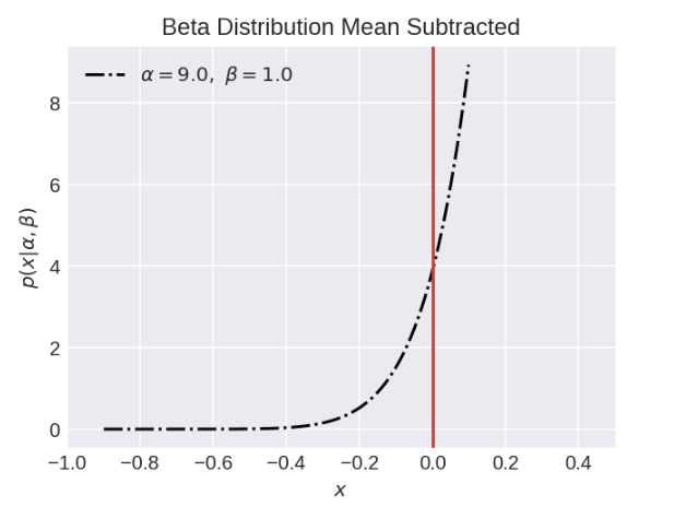
If we sum all values of our deviations we do in fact get 0. Thats because there are a few large deviations to the right but many smaller deviations to the left. When we sum them, the smaller values occour with a much higher frequency so they are able to cancel the larger values. If expected winnings of a game are 10$ $ $, and I subtract 10$ $ $ from each game, then I expect to win 10-10=0$ $ $ per game($E[X-E[X]]=E[X]-E[X]=0$). So once again, the mean is the point around which the positive and negative deviations cancel out.

— I want this idea to stick that the sample mean in a sample has deviations sum zero. Now lets

Let’s rewrite the mean formulae with this insight. We will now consider a very very large number of sample so that

1) $\sum d_i \approx 0 $

2) So that we equate this to the true population mean $\mu$ as the defination states:

$lim_{N\mapsto \infty} \frac{\sum_i^Nx_i}{N}\mapsto \mu$

We will write each $x_i$ as how it deviates from the sample mean as before. We use the sample mean as we generally don’t know the true mean but we do know the deviations around the true mean approximately sum to 0. This small deviation becomes part of the sample mean so it is a slightly biased estimate of the true mean. So x bar and mu differ slightly. Thus x bar - di is really like mu-di+error So we are considering the sample mean as the true mean then $\sum d_i \approx 0 $ only when we take the mean of the points under consideration.

We will express each x as some deviation from the true mean: x_i=\mu + d_i. Earlier we represented each point as a deviation from the sample mean and those deviations summed to 0. But here \sum d_i won’t be exactly zero due to the randomness of sampling. (out sample is a approxiamtion of the true frequencies) \(\frac{\sum x_i}{N}=\mu\)

\[\frac{\sum (\bar{x} + d_i)}{N}=\mu\] \[\frac{\sum \bar{x} + \sum d_i}{N}=\mu\]

If we were taking large amount of samples we would expect the positive and negative deviations to almost cancel each other out in the long run so $\sum d_i \approx 0 $

\[\frac{\sum \bar{x}}{N} \approx \mu\]

And as $\bar{x}$ is a constant $\sum \bar{x} = N\bar{x}$ giving

\[\bar{x} \approx \mu\]

This is saying taking a large number of samples, we expect the sample mean to be a very good approximate of the true mean beacuase we expect the deviations around the mean to cancel each other out. When the deviations cancel each other out, we are left with the only consistent signal in the distribution which happens to be the mean. (think about it using the experession $lim_{N\mapsto \infty} \frac{\sum (\bar{x} + d_i)}{N}$, if the $d_i$s keep cancelling each other they will get swamped by the every growing N)This idea of thinking in terms of how the sample mean would deviate from the true mean will provide us critical insight into the guassian distribution. In the case of the uniform it was quite straight forward, in the case of the gamma if the sample has frequencies that concur with the true frequencies given by the analytical distribution then we expect the smaller deviations occuring in their larger frequency to cancel out the larger ones occuring in their smaller frequency leaving only the mean as a consistent source of signal in the summation term.

Thus he concluded by saying, “If observations of all events be continued for the entire infinity, it will be noticed that everything in the world is governed by precise ratios and a constant law of change.” This idea was quickly extended as it was noticed that not only did things converge on an expected average, but the probability of variation away from averages also follow a familiar, underlying shape, or distribution.

In the real world we see that not only do things follow patters, but even deviations from those patters follow patterns themselves. Thus statistics is the study of not only patterns, but even the behavior of the deviations from those patters. This will motivate us to study the approximation \(\bar{x} \approx \mu\).

Here is a paraphrased version of one of my favorite explanations of anything ever. It is taken from chapter 4 of Statistical Rethinking By Richard McElreath:

Normal by addition

Any process that adds together random values from the same distribution converges to a normal. But it’s not easy to grasp why addition should result in a bell curve of sums. Here’s a conceptual way to think of the process. Whatever the average value of the source distribution, each sample from it can be thought of as a fluctuation from that average value. When we begin to add these fluctuations together, they also begin to cancel one another out. A large positive fluctuation will cancel a large negative one. The more terms in the sum, the more chances for each fluctuation to be canceled by another, or by a series of smaller ones in the opposite direction. So eventually the most likely sum, in the sense that there are the most ways to realize it, will be a sum in which every fluctuation is canceled by another, a sum of zero (relative to the mean).

It doesn’t matter what shape the underlying distribution possesses. It could be uniform, like in our example above, or it could be(nearly)anything else. Depending upon the underlying distribution, the convergence might be slow, but it will be inevitable. Often, as in this example, convergence is rapid.

It’s hard to say where any individual person will end up, but you can say with great confidence what the collection of positions will be. The distances will be distributed in approximately normal, or Gaussian, fashion. This is true even though the underlying distribution is binomial. It does this because there are so many more possible ways to realize a sequence of positive negative steps that sums to zero. There are slightly fewer ways to realize a sequence that ends up plus or minus one, and so on, with the number of possible sequences declining in the characteristic bell curve of the normal distribution.

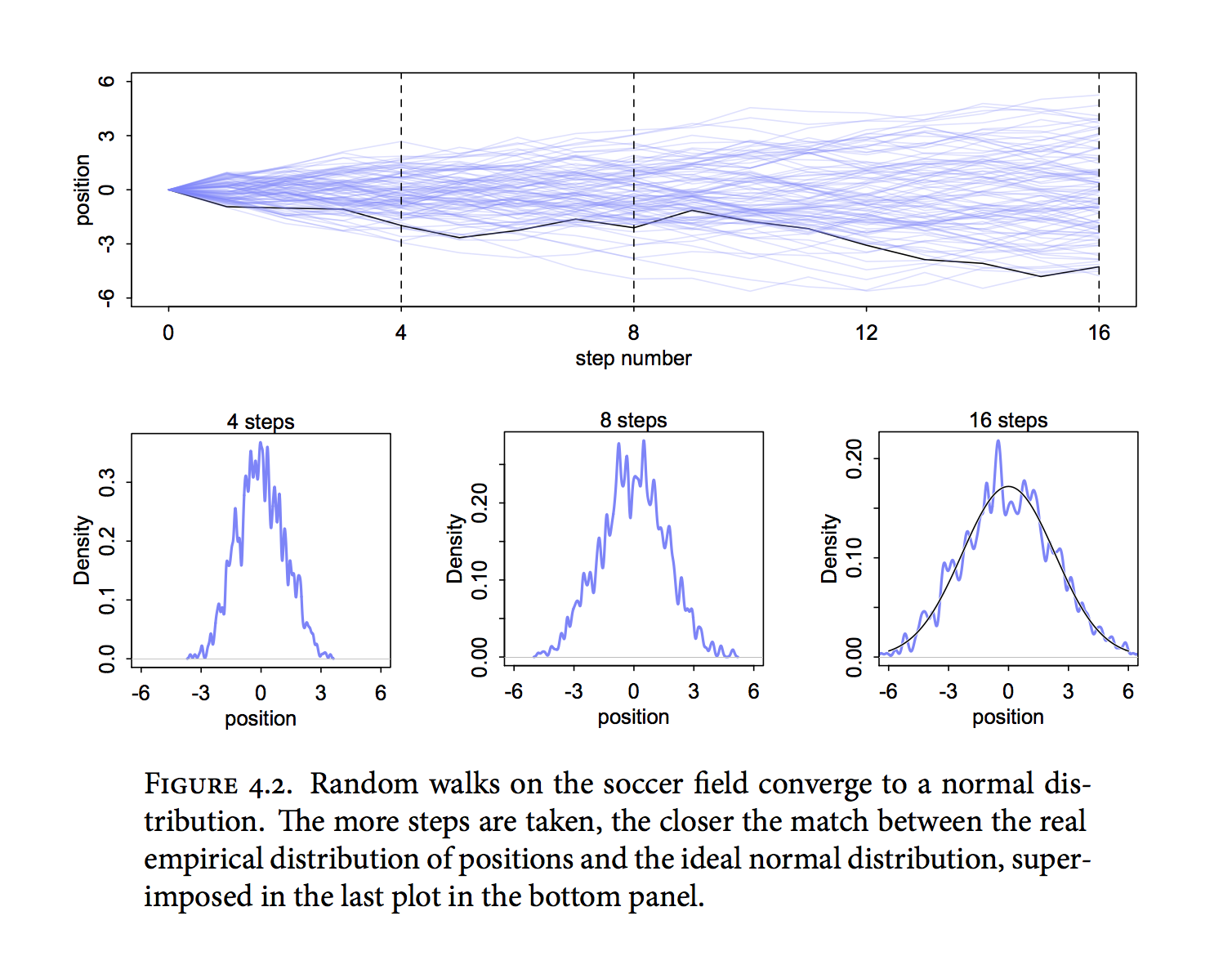
We will simulate a very similar example to this image, but remember our aim is to describe real processes and not cute mathematical abstractions. But the fact is that the additive behavior of deviations that we have been describing occurs alot in nature and it is this process of addition that leads to the shape of the bell curve. And if you can understand things about how this addition occurs, then you will understand why the bell curve is the way it is. We are trying to realize things about this bell curve by studying the additions that caused it, and luckily the additions are way more simple to understand that looking at the bell curve directly. Usually the fact that the CLT applies to any distribution is lauded and called a marvel but when we saw that even the deviations of non-symmetric distributions cancel each other we already proved this trival fact.

– statesmenrts about considering x-di makes it independant of distribution, how CLT is about deviations and not true values in the dist. My CLT implies CLT

– new heading [We want to reslly understand the connection between the mean and deviations so lets:] Let’s consider a binomial distribution with p,q

– We give this example of coin toss and show how it is equivalent to error obersvation around 0(Gauss and astromical measurement). this example will provide a base to undertand the distribution of errors – consider an illuminating example

The next example is identical to how we can treat errors in the random world: as a fluctuion acting on the true signal. We will use the very practial(and discrete) example of a coin tossing game and later connect this this to the continous(and overwhelming) case of random errors. In this game if the coin is heads I win 1\(and if tails I loss 1\)

The expected value of the game can be computed as : $E(X) = \sum xp(x) $ $E(X) = (1/2)(1) + (1/2)(-1) = 0 $

Which is saying in the long run sum of +1’s and -1’s(+1 -1 +1 +1 -1 +1 +1 -1 +1 +1 -1 +1 -1 …..), all +1s will cancel the -1s. Consider 10 trials, in the expected senerio there would be equal number of +1 or -1 so our net winning would be 0. However in the real world we could have got 6 heads and 4 tails or 7 heads and 3 tails. If N=100 our potential winnings would range from +100 to -100. But +100 seems pretty rare right? I would have to get all heads for that. I bet you that’s its more rare than +50. Can you think why this would be the case?

What about for smaller values? Is +2 more rare than +1? or -3 than -2? This is a good time to use some of our previous work and think about this.

What we want to argue here is that +2 is less likely than +1 and -2 is less likely than -1. The farther the winning is away from the expected value of 0, the less likley it is. And since this game can can be expressed as a binomial distribution we are in good luck.

We can model a single toin coss as a Bernoulli distribution and a set of tosses as a Binomial distribution with $N$ as the number of tosses:

$X \sim Bn(p=1/2,N)$

$P(X=x)=\binom{N}{x} p^n(1-p)^{N-x}$

$P(X=x)=\binom{N}{x} (1/2)^x(1/2)^{N-x}$

$P(X=x)=\binom{N}{x} 1/2^N$

We can plot this for different values of $N$ and see the probability distribution of how many heads we get. If $x$ is the total number of heads observed then $N-x$ is the total number of tails. We can now visualise how likely different pair are and see if we observe any pattern.

We see that in all the cases, the shape of the distribution follows a familar pattern. Let’s plot the expected winning distribution as well. If I get more heads than tails i.e if $x>N/2$ I make a profit and vice verse. The profit we make is proportional to the number of heads and vice versa. At $x=N/2$, we have 0 profit. The next plot should not suprise you.

We see that the most likley number is $N/2$ (remember $N/2$ corrosponds to the case of equal heads and tails and winning of 0). And values away from that becomes less and less likley. The relationship is strictly monotonic in the left and right regions. This is a key point we will exploit later. #You can pause and think why this would be the case.

As the quote stated earlier “there are so many more possible ways to realize a sequence of positive negative steps that sums to zero”, now remember zero meant the expected value in all our cases as we mean subtracted the distribution. In this case the mean is really zero so we already satisfy this condition. In this example $\binom{N}{x}$ term is maximized in our binomial distribution at $x=N/2$(which is the same as expected winning of zero). If you remember this term gets added when we go from Bernoulli to Binomial to count the number of ways an outcome can now occour. So if $N=4$ the possible pairs are $(1,1),(1,-1),(-1,1)$ and $(-1,-1)$ but observing $(1,-1)$ is the same as $(-1,1)$ for us as we dont care about ordering so this gets accounted in the factor $\binom{2}{1}=2$. And this is true for large numbers as well. So the reason why $N/2$ is most likley number of heads or why a winning of 0 is most likley is because in N tosses the number of ways I can sum +1 and -1 to equal 0 is more than the number of ways I can use them to get any other number and ways I can sum +1 and -1 to equal +1 is more than the number of ways I can use them to get +2.(Think about how this is implied in $P(X=x)=\binom{N}{x} 1/2^N$ when $N$ is fixed, the only variable is the counting term)But anyways I hope it was already quite intutive to you from the setting of the game that small winnings/losses were more likley than large winnings/losses, we have just shown this is a result of counting operations.

We will summarise this important result, which we will later see applying to measurement errors, as :

A) Small winnings are more likely than larger winnings

or

A) Values close to the mean are more likely than those furthur away

In the example of $N=50$, $x=24$ corrosponds to to -1$ profit and $x=26$ to 1$ profit. Due to the symmetry of the counting factor : $\binom{50}{24} = \binom{50}{26}$

Or generally $\binom{N}{x} = \binom{N}{N-x}$

So the distribution is symettric. We summarise this as:

B)For any real winning $a$ the likelihood of winning a and −a are equal.

In a way we can consider zero to be the true signal of the game. Its the real expected value in the long run and +1’s and -1’s are noisy signals which cancel each other out. If you’re not convinced with the statment keep reading.

Consider a very small extension of the above experiment and then we can move onto errors. What if I won 51 at every heads and 49 at every tails. What would be my average winning?

Lets write the above game in terms of deviations as we did before

\[\frac{\sum x_i}{N}=\frac{\sum (\bar{x} + d_i)}{N}=\frac{\sum (50 \pm 1)}{N}\]

$=\frac{\sum 50}{N} + \frac{ \pm 1}{N}$

$ = 50 + \frac{+1 -1 +1 -1 +1 -1 +1 -1 +1 -1 +1 -1 ….}{N}$

Notice how the second term is exactly like our first game! A winning of +1 and -1’s around 0 is now a winning of +1 and -1’s around 50. This shows more clearly the statement that the mean, 50, is the only consistent source of signal in game while +1 and -1’s are random fluctuations than act upon it.

The graph of this is

Or

Great job getting this far! Now I would like to c

Random Errors:

Imagine you are Carl Friedrich Gauss out in the woods with you telescope trying to measure the distance between Earth and Ceres:

You simply wanted to find out this distance but every time you record a measurement, you get a slightly different value. Sometimes its really different from the rest and sometimes it almost the same. You have no idea what to do or which one to consider as the true value. This was the case with much of astronomy in the 1800s. So which one of these measurements should you take to be the true value for your very important calculations? # pause and appreciate this dilemma

Well, lets first ask why we are getting different values in the first place. Your telescope is extremely sensetive to slight changes in movement.

–slight change to angle

There are various sources that could be the case for different measurments like the telescope being wobbly, wind moving the telescope, uneven surface, instrumental error, measurement reading error and so on and so forth.

There could be a finite number of classes for errors, but you will agree that the forces causing those errors is infinite. So there are a gazillion air particles acting on the telescope vibrating it very slightly. These particles are unbiased, meaning they have no special preference to increase or decrease you measurment. Your telescope is equally likely to be tilted left or right. Each particle adds a unit of force in some direction and particles on one side of the telescope cancel the effects of particles on the other. Does any of this sound familiar?

This is exactly the situation we had earlier with the coin tossing example. Except here the coins are particles, heads are particles pushing us to the right and if we are being pushed more to the right than left then our movement is a postive unit in the right direction. If the errors caused by the wind were truly random fluctuations then their expected movement on the telescope is zero because they have no preference in which direction to push(think maximum entropy). If there is a preferance, then it is a source of systematic, and not random, error.

Now if we strip all causes of error to their individual units of forces, each having no preferace into which direction to push the telescope, then we have a case of infinite elements each with equal probability of heads or tails …. I mean equal probability of pushing the telescope to the right or left. This is essentially a binomial distribution with $N=\infty$ which decreases from it’s expected value in the characteristic way shown above. But now that there are so many errors, this curve’s range on the x-axis is much much broader than shown above, leading to vastly different values at each observation.

This is just assuming we can only move right or left, but if we could also move up and down or other angles, then you could imagine we would have similar looking curve but in higher dimensions.

So the level of wind at any point is a cause of a very large number of particles and their interactions. A few of these forces may influence the wind in the one direction and a few in the other.

I’m using could be a bit wobbly so each time it is affected by my hand pressure. The wind may also be blowing fast and slow vibrating my instrument. The grass may be uneven chaging my angle very slightly. There could be some instrumental error due to accuracy limits of my telescope. Measurment error in me reading the non-digital(its the 1800s after all) readings and so on and so forth.

Consider an unbiased error, an error that that has a chance of increasing or decreasing you measurment equally. If

These forces have no rhyme or reason to favor your measurement in any direction. They are random or unbiased.

• consider these +1, -1 as errors and we are not infinitely adding them

We have the case of Normal like curves for single cases of uniform and binomial. Let’s get a little furthur. First, lets restate our defination of the mean. When thinking about the mean, it helps greatly to consider the pracitical reason why its invention was necessary.

Our first defination of the mean stated “the mean is the number around which the deviations are perfectly symetrical and cancel each other out”. But the deviations won’t always be symetrical for non-uniform distributions.

\[\frac{\sum x_i}{N}=\mu\] \[\sum x_i=N\mu\] \[\sum x_i-N\mu=0\] \[\sum (x_i-\mu)=0\]

From this we can see that the mean is the number from which all the negative deviations and positive deviations sum to 0.

Consider the set (1,1,1,1,99). The mean here is 20.6 and the $d_i’s$ are -19.6 for the ones and +78.4 for 99. If we add all the x’s expressed as $x_i + d_i$ we would get 5(20.6)-4(19.60)+78.4=5(20.6) The mean is the value from which the magnitute of deviations to the left and right sum to 0.

The summing operation over the values leads to N$\mu$ because we expect the deviations to cancel out, the mean is the only thing that contributes to the sum. If I just told you the mean of a distribution and told you I have sampled K points, you could guess the sum of those would be K$\mu$ and you would’nt be too far off. So suppose we observe some phonemeon that is additive, like random noise. Say there are 100 sources of noise in a measurement each capable to being +-1. At any time all these act, so we can expect the net sum to be 0.

$\sum(x_i - \mu )=0$

If every x_i has the same probability but if x_i has some other distribution like there are 98% 1’s and 2’s and 2% 99’s then sums of the deviations of 1’s and 2’s should cancel out the deviation of 99’s.

-mention limiting case of binomail is normal

–Quote from statistical rethinking about normal

Or in other worlds : large deviations are less likely than smaller ones.

[ CLT:The central limit theorem states that the distribution of sample means approximates a normal distribution as the sample size gets larger (assuming that all samples are identical in size), regardless of population distribution shape.

We say the distribution of total deviations in normal. And this implies ^ ]

Consider only 10 points from this distribution from simplicity