Signal Processing of speech and audio files

---

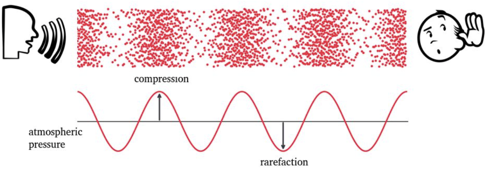
2- Sound and waveforms

Air molecules transfer energy through space, not molecules themselves. The variations in air pressure of create the perception of sound.

We can categorise these waveforms into multiple types as

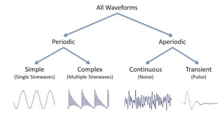
In a simple waveform if T is period taken from one peak to the next then freq = 1/T Hz Phase is the angle we shift during the start. So at x=0 , y= sin(x+-phase) Humans perceive high frequency sounds to be louder, even if amplitude is the same of two sounds. Humans can hear between 20-20,000Hz

Pitch is human perception of frequency, they are correlated but humans perceive frequency in a logarithmic way. If a frequency differs by a power of 2 then we think they sound similar. Basically if one was 10 Hz, and the other is 20Hz then the 20Hz is seen as a faster version of the 10Hz. The waveform is just twice as condensed. However 15 Hz is felt to be qualitatively different, it is not perceived as 1.5 times faster. 40Hz is considerd similar to 20 Hz and so on. So by powers of 2 we notice similarity(what about 30 Hz vs 10 Hz, not 3X faster?)

The pitches A3 (220 Hz), A4 (440 Hz), and A5 (880 Hz) sound similar. Furthermore,the perceived distance between the pitches A3 and A4 is the same as the perceived distance between the pitches A4 and A5. In other words, the human perception of pitch is logarithmic in nature.

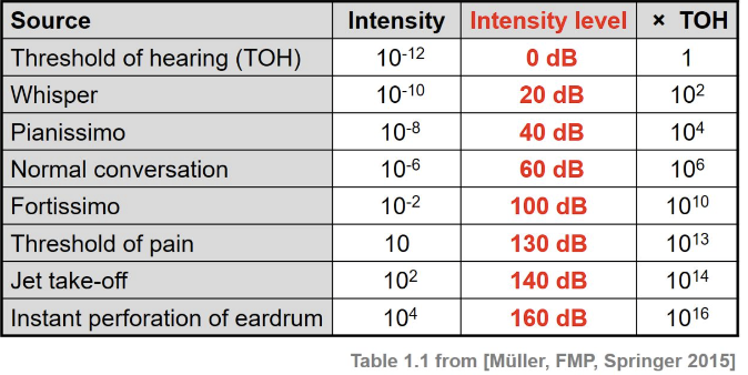
3- Intensity, loudness, and timbre

Intensity A thunder and an oristra only produce 1W of sound where as a bulb is 100W. We can percieve sounds from our threshold of hearing(TOH): 10^-12 to 10 W/m^2 which is 12 orders of magnitude! Intensity(I) is measure in this unit as W/m^2 Decibal of a sound is then calculated based on a base TOH: \(dB=10log(I/TOH)\)

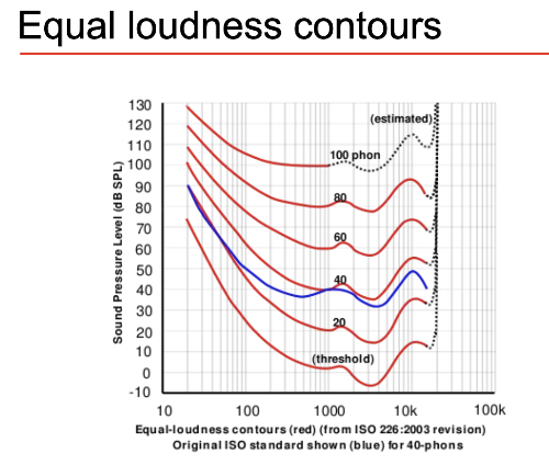
Loudness As humans perception of loudness is influenced by amplitude, frequency and duration. High amplitude with less duration or frequency is percieved as less loud. Abstract measure of Loudness is phon. Plot of freq vs intensity shows contours of constant perception.

Timbre Sounds with same amplitude/frequency have different waveforms which produce qualitive differences in sound.Each sound wave has a characteristic shape, which depends on the material that produced the sound. This is what defines the timbre of the sound.

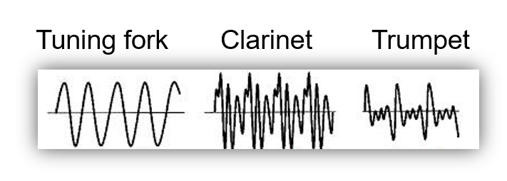
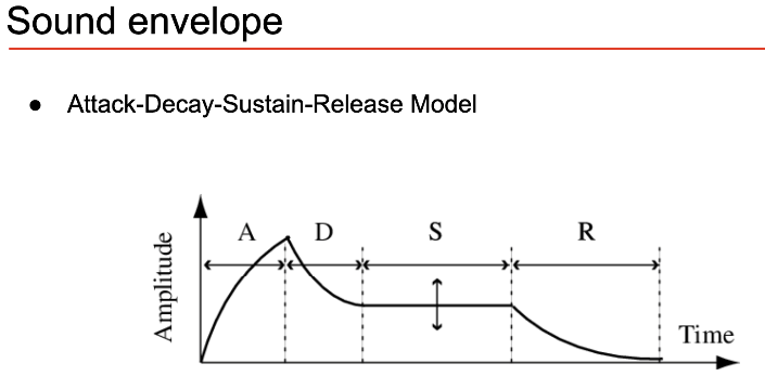
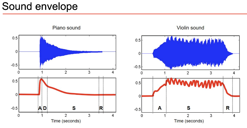
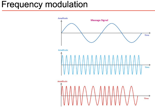
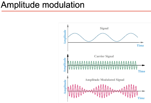
Timbre has 3 major features: Sound Envelope, Harmonic Content and Amplitude/freq modulation

Sound Envelope See Fundamentals of Music Processing by Muller for more.

Complex Sound is the fast fourier transform Amplitude/freq modulation: deliberate modulation

4- Understanding audio signals Sound is a continuous and infinitely precise object. To represent it in a computer we have to sample and quantise its values. Sampling

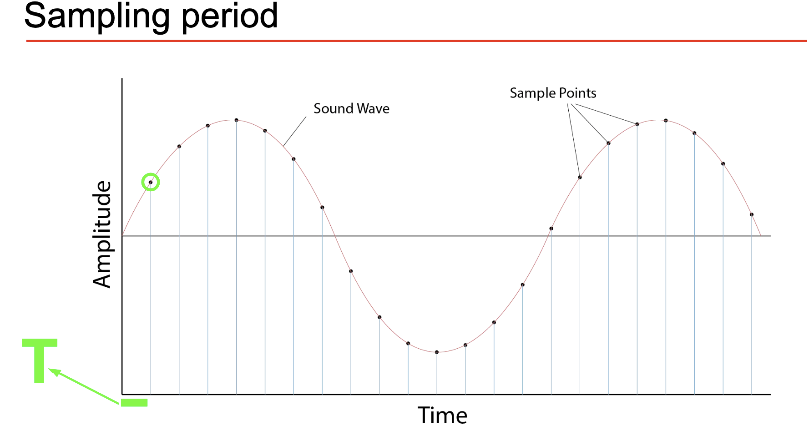
The sampling rate is \(s_r=1/T\) which measures number of measurements in 1 sec

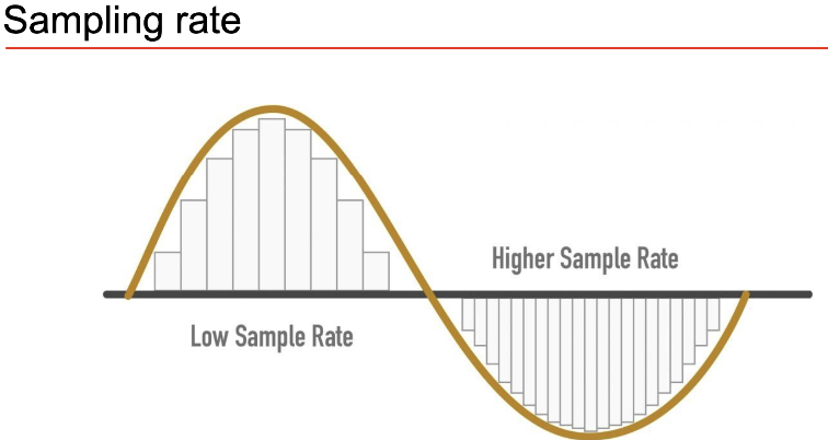
If we measure at 40% the freq then we will measure at 40%, 80%, 120% 160% .. giving a jaggy wave. See Nyquist Frequency which is \(s_r/2\) which says the max freq we can measure without artefacts like aliases Sampling rate for a CD is 44,100Hz which has Nyquist Frequency of 20 000 Hz which is max human hearing range. So CD can produce whole human hearing range.

Quantization

A regular CD has 16 bit precision with sampling rate as above of 44,100. So 1 minute of sound will consume:

total bits = 16*44,1000 ; 1,048,576/8 bits= 1 MB

=>16*44,1000/(1,048,576/8) = 5.49 MB

See dynamic range and signal to quantisation noise ratio

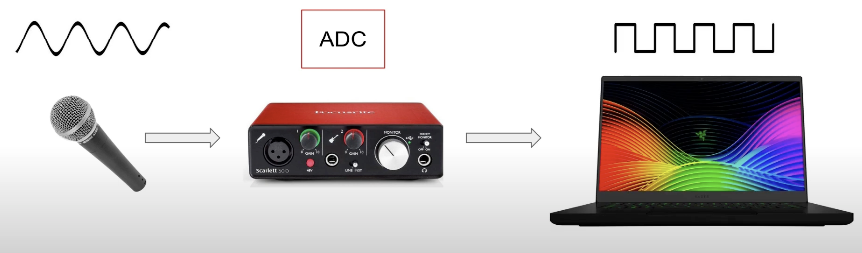
Analogue to Digital Converter does sampling, quantization, Anti-aliasing: low pass filter that cuts all frequencies above Nyquist Frequency

5- Types of audio features for ML

Humans need atleast 10ms of audio to make sense of. That’s why we generally chose segments>10ms(?)

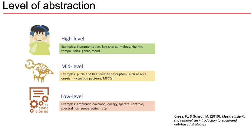
Audio feature categories 1) Level of abstraction - More for music signals. Low-level are non human understandable, statistical features - Mid-level are more perceptual - 2) Temporal Scope - Features on different time intervals: Instantaneous(~50ms), Segment-level(seconds), Global

3) Music Aspect - For music: beat, timbre,pitch, harmony ….

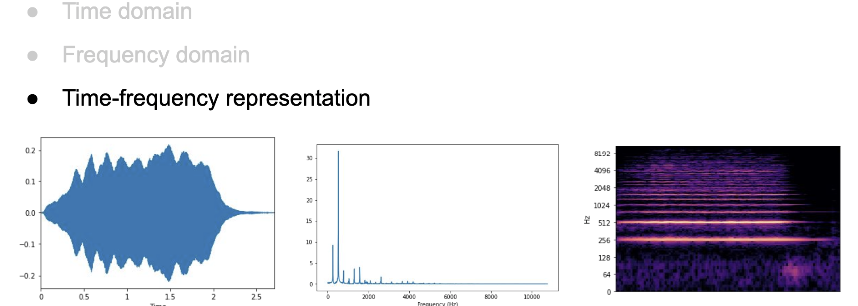
4) Signal Domain

Time, Frequency, Time-Frequency features(see names of time/freq features in slides)

5) ML

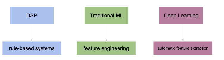
6- How to extract audio features

We see the three types of features: Time, Frequency, Time-Frequency above

Time domain: For Time domain we can split the timeframe into overlapping chunks and calculate feature for each of those chunks and then aggregate all for a complete representation 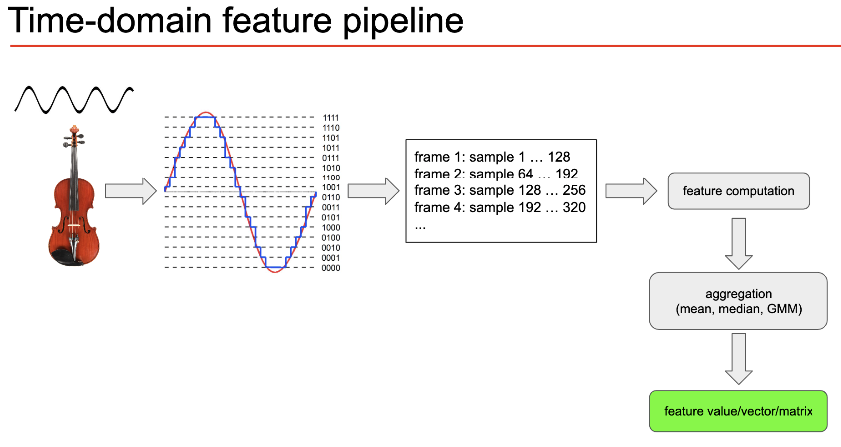Frame size : We typically want our frame size to be human perceptible(10ms) so features make human sense. So if the sampling rate is 44,100 Hz i.e 0.0227ms/sample we normally take 512 points(typically 256-8192) leading to a frame duration of 0.0227*512=11.6ms. Frame size: We typically want frame size to be a power of 2 as it makes fourier transfrom faster to compute

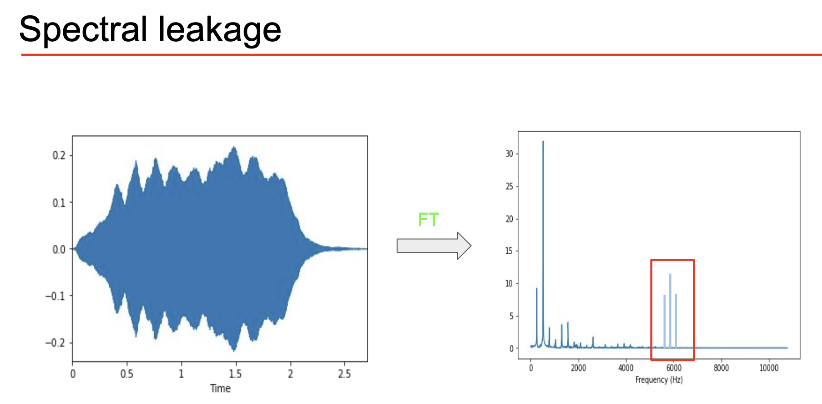
Frequency Domain: We want to compute frequency features by taking the fourier transform of our frame sets However if we compute fourier transform of a signal which non-integer number of periods in the frame then our transform will add all bunch of non-existent frequencies to match the fractional frequency at the end as it is just curve fitting. If it was an integer then things are straightforward. This is called __Spectral Leakage.__ 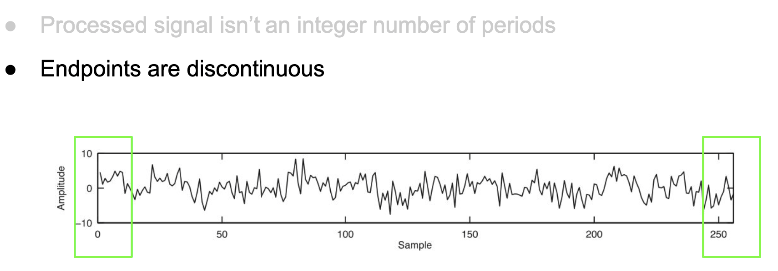As end-points are discontinuous, they are thought to be high frequency patterns
Discontinuities appear as high-frequency components not present in the original signal Hann Windowing 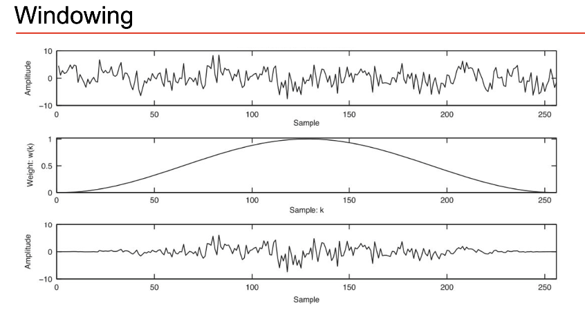However if we apply this to each individual frame we loose alot of info on corners

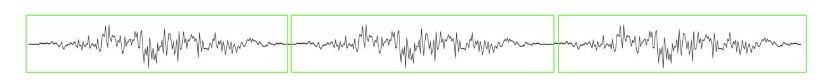To overcome this we use overlapping frames so every part of the signal is measured

7- Time-domain audio features

Some time-domain features: Amplitude envelope (AE): max amplitude value - 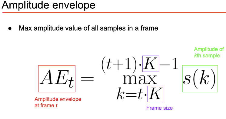- Gives rought idea of loudness but sensitive to outliers -

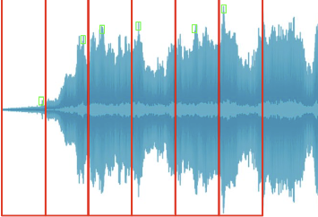
We can use this to detect onset of some musical note or classify music generes

Root-mean-square energy (RMS): sum of square values - \(R M S_{t}=\sqrt{\frac{1}{K} \cdot \sum_{k=t \cdot K}^{(t+1) \cdot K-1} s(k)^{2}}\) - Less sensitive to outliers - Identify new segments in audio as audio changes alot, music genre classification

Zero-crossing rate (ZCR): number of times of zero crossing - 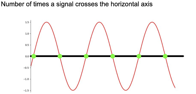- \(Z C R_{t}=\frac{1}{2} \cdot \sum_{k=t \cdot K}^{(t+1) \cdot K-1}|\operatorname{sgn}(s(k))-\operatorname{sgn}(s(k+1))|\) - Identify percussive(random) sounds vs pitched(structured) sounds - Voiced signals have lower ZCR than non voiced so can use to identify that