Understanding the Perceptron
Understanding the Inner Workings of Neural Networks
In this post we shall understand how neural networks or Multi-Layer Perceptrons(MLPs) make sense of input features and repurpose them to solve the task at hand. We will use the powerful abstraction of logical operators to make networks more intuitive and easily interpretable. Everything in this post can be applied to more complex use cases and higher dimensional feature spaces.
The Single Perceptron:
A single perceptron is just a weighted linear combination of input features. Suppose we have inputs \(x_{1}, x_{2}......x_{n}\) and corresponding weights \(w_{1}, w_{2}......w_{n}\). Then the dot product of these two vectors can be represented by:
\[\sum\limits_{i=0}^{n}{x_{i}w_{i}}+b\]We can think of the weights as the degrees of importance attached to each input feature. If more favourable features are present then the dot product will be higher. Therefore the linear combination gives us a score for what we are looking for. The bias term acts as a threshold, we shall see this further.
The common symbol for this linear weighted sum in network diagrams is:

Representation Power
We can show that a single perceptron, or less formally, a single weighted linear combination can act as a logical gate. In order to do this we include an activation function, which in this case is the step function:
\[\begin{eqnarray} \sigma(z) & = & \left\{ \begin{array}{ll} 0 & \mbox{if } z \leq 0 \\ 1 & \mbox{if } z > 0 \end{array} \right. \end{eqnarray}\]So our perceptron can now be written as:
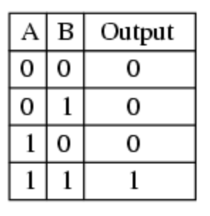
\[Output=\sigma (\sum\limits_{i=0}^{n}{x_{i}w_{i}}+b )\]The AND Gate Let us consider two inputs features \(x_{1}, x_{2}\) which can either be 0 or 1 indicating absence or presence. The AND gate outputs a 1 if both inputs are 1 and 0 in all other cases. Our job is to find \(w_{1}, w_{2}\) and b so that our perceptron behaves the same way.
The AND Gate looks like:
The perceptron looks like : \(\sigma(w_{1}x_{1}+w_{2}x_{2}+b)\)
As \(x_{1}, x_{2}\) are desirable features we start by giving them positive weights of \(w_{1}, w_{2}\)=1.By playing around a bit we observe:
- \(x_{1}, x_{2}\)=1 \(\Rightarrow\) Output = 2
- Either \(x_{1}, x_{2}\)=1 \(\Rightarrow\) Output = 1
But since we want the second sum to be negative so that our step function can reduce it to 0, we make use of the perceptrons’s thresholding factor and set b = -1.5
So now our outputs are all exactly as the AND table. The bias is effectively saying “Some of the features I am looking for are present but not enough”. The whole concept of thresholding can be summed up by the previous line.
The OR Gate

Now consider the OR gate. The OR gate activates when atleast of the features is present. Since the OR gate just has less feature requirement, we can construct an OR gate by reducing the bias. We set b = -0.5.
The NOT Gate A NOT gate simply takes an input, \(x_{1}\) and inverses it. 0 become 1 and 1 becomes 0. This can be done as \(-x_{1}+1\)
If we pass our outputs from an AND gate to a NOT gate we have effectively created a NAND gate. A NAND gate is considered a universal gate i.e any logical computation can be computed only using a combination of NAND gates. Hence our single perceptrons can be combined for exactly the same behavior. (You can play around with logic gates a bit more at Lesson 2.8 of Udacity’s Intro to Deep Learning with Pytorch course for free)
We considered a simple case of two input features, but with many more features, a combination of perceptrons can form intricate logic conditions for the task at hand. We can construct multiple layers of perceptrons to make more and more elaborate compositions of logical operations in between the inputs. That network would look like:

A perceptron in the \(N^{th}\) layer does a weighed linear combination all the outputs of the \(N-1^{th}\) layer. As it computes another logical operation on all the operations already computed by the \(N-1^{th}\) layer, it is able to form a deeper operation with respect to the inputs. This is what is called a Multi-Layer Perceptron(MLP) or Neural Network.
Logical gates are a powerful abstraction to understand the representation power of perceptrons. We shall see more examples of it below. But as we move to continuous inputs and outputs we can more fully understand how MLPs are used for a range of modern tasks through the lens of two important functions: ReLU and Sigmoid. In modern architectures, ReLU’s are used inplace of step functions and Sigmoid is used on the output of the MLP.
Relu
Usually in MLP’s, ReLU’s are used instead of the step function. A ReLU is defined as :
\[\begin{eqnarray} \sigma(z) & = & \left\{ \begin{array}{ll} 0 & \mbox{if } z \leq 0 \\ z & \mbox{if } z > 0 \end{array} \right. \end{eqnarray}\]Or more compactly: \(\sigma (z)=max(z,0)\)

The only difference from the step function is that it lets positive values remain as themselves. ReLU’s allow us to break free from the discrete outputs of the step function and allow us to compose a plethora of functions by stacking them together. Let us say we have the task of estimating some value, maybe the house price based on various inputs. In this case, our output cannot just be 0 or 1 but some number. This regression problem can be solved by finding an appropriate function \(h(x_{1}, x_{2}......x_{n})\) which outputs the price based on the input features of the house and market. We show that such a function, in fact any such function, can be estimated by using a bunch of ReLU’s each contained in one perceptron. ReLU’s can even be used for classification problems as they divide the space into distinct parts, we’ll see a concrete example of this soon.
Consider a MLP with one input and one hidden layer with two perceptrons. Each perceptron(P) will assign some weight and bias to the input and output a ReLU function as \(P_{i}=\sigma(w_{i}x_{1}+b_{i})\). Example:

The output node will then take a weighted sum of these two functions as \(W_{1}P_{1}+W_{2}P_{2}+B\) :
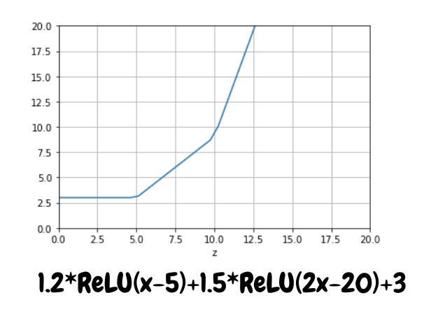
By the next plot I hope you will be able to see the power of ReLU in approximating any function :

This looks alot like \(x^{2}\) doesn’t it? The Universal Approximation Theorem says that an MLP with enough perceptrons in one hidden layer can approximate any function to an arbitrary degree of accuracy within a bounded region. Boundedness is a very important concept for any machine learning model but we look over it for now. Because we can pick up and place a ReLU anywhere by adjusting the thresholding factor or bias in each perceptron, we can simply stack ReLU functions side by side(you may be able to notice the dents in the \(x^{2}\) plot above where one ReLU just began).
In essence, using ReLU gives us the total power to change the gradient of our function at any point by adding a ReLU with the appropriate increase or decrease slope. If we have total control on the gradient, we have total control over what we want our function to look like as we can effectively steer it in any direction at any speed we like from any point onwards. This post has some great replies for more reading. This same concept applies in some N-dimensional space; with more inputs ReLU’s can approximate any N-dimensional surface to arbitrary accuracy.
ReLU’s can also be used for classification problems. This is because ReLU’s form a straight line seperating two regions of space. In the first plot of the ReLU function we can see it has seperated the graph into a region where \(x>y\)(below the ReLU line) from \(x<y\)(above the ReLU line). And it has seperated the two subsequent graphs through some other function. We can use this space seperating feature of ReLU along with logical gates to create a powerful classification algorithm. Suppose we have one hidden layer with 4 perceptrons.
How could we solve the following classification problem? Pause to figure it out. You know enough! Or scroll down just a bit for a hint.

2 pair of neurons each would combine to mark out the regions of intrest as :

In both, two ReLUs have seperated the space seperately according to their own criterias and then an AND gate has been applied to get the common space that meets both criterias.
And then ? Pause to try and figure it out….
.
.
.
Then we simply pass this into an OR gate at the final node and our classes have been distinguished!

Two more examples:
Have a look at this example from TensorFlow Playground:

Just click play and you’ll see a solution being formed. The network forms a different solution each time depending upon how the weights are initialized. In the first one, 3 perceptrons corner the Blue region(look inside each neuron to see its positive and negative region) from three sides and the final node applies an AND gate(easily inferred from the last output) to all the three. The second trial found one inverse region to apply a NOT gate to(look at the first neuron in this one). The sign of the weights can be made out from the color of the connections shown and the weights can be seen by clicking each perceptron.
Consider this example:

Here we see the power of more than one layer. The first layer, as it is only applying a single ReLU function, is able to spereate the space with only one line at each perceptron. But the each of the next perceptrons takes all the inputs of the first layer to form more intricate patterns(look inside or hover over each perceptrons to see these region). The first layer is optimized to give the best inputs into the next layer.
Using the abstraction of logic gates in these examples made it extremely easy to see how our model could divide the data and what it would do in the end. We can apply this same abstraction to scenarios where we have many more features to reason what our network is doing. For example, in a CNN the decision node in a dog detector may look something like : Nose AND (Pointy Ears OR Sharp Ears) AND Eyes AND Tail NOT (Glasses OR Clothes). In fact, these decisions are not strictly binary, but continuous as each sub-operation in a single logical operator contributes some score(based on its weights) to the logical operator. So we get an output of how much the pattern being looked for is persent or absent. If it is present in enough amounts we say the perceptron is ‘firing’.
Think about any such intricate logic, no matter how convoluted, and MLP’s can mimic it. Each layer will create operations which will help the next layer create better operations in a pyramid-like fashion to solve any intricate problem. That’s pretty powerful! But what makes MLPs even more powerful is that not only can they apply these logical operations on features but they can construct their own features in the hidden layers on which to apply their operations on! Woof ! Let that sink in for a bit.
Let us think about why Geoffrey Hinton believed for so many decades that neural networks could mimic decisions made by the brain. Consider a buyer rating a car from a scale of 0-10. There would be some factors like price, mileage, pick-up, comfort, brand etc that a buyer would look at to rate a car. There is a different degree of importance he places on each of the factors. This function in the buyer’s mind is very approximately linear. Think about it! Think about the way you may rate your favorite sports player or games or even peers. Decisions are very approximately linear except maybe at the very hign and low ends of the scale. As we know this can be represented by a single neuron. But now suppose I told you to rate sports cars instead of regular cars, your function would change alot. You may not place the same importance on brand and alot more to the stats of the car. The same if I told you to rate a jeep, buget or a luxuary car. What you have is a whole collection of inernal approximately linear functions ready at your disposal according to the situation. We can represent these many functions as a layer in a neural network. Now if I show you just pictures of random cars, you would first decide which type of car this is and the use the rating function assoicated with that. So there a an extra layer of preprocessing you do. We can represent this is layer 1 and the rating functions of the car as layer 2. These type of nested decisions along with non-linearities are the reason why neural networks were thought to be able to mimic brain decision very well. In face you should spend some time thinking about how unexpectedly(and approximately) linear so many of your decisions are. You would be suprised!
Sigmoid
It is important to have a sense about how the sigmoid function works. Sigmoid functions are used on the outputs of MLP’s in binary classification problems where we have two possible classes; telling whether an image is of a lion or giraffe is such a problem. Sigmoid outputs a value between 0-1 that can be interpreted as the score or probability of one of the classes.
The sigmoid function is defined as: \(\begin{eqnarray} \sigma(z) = \frac{1}{1+e^{-z}}. \end{eqnarray}\)

We use the sigmoid in place of our step function at the end as instead of just outputting a 0 or 1 it gives us a score for how favorable our desired event is. If we are a little favorable, then we may get 0.55 and very then 0.95. Another great property is the sigmoid is differentiable, this will be useful for optimizing the network.
If a class has a probability higher than 0.5 we pick that class. We pass in the network output \(z\) into the sigmoid function and see what must it satisfy for class 1 to be selected(as opposed to class 0) :
\[\frac{1}{1+e^{-z}} >0.5\] \[e^{-z}>1\] \[z>0\]i.e \(z=0\) is the equation of the decision boundary line/curve where input features show equal evidence of either class. Now as \(z\) is the output of the neural network it must be greater than \(0\).
We can show that for a single perceptron this means the sigmoid creates a line dividing the examples.
Proof:
Say, we are camping in the jungle and hear some footsteps at night. We want to classify if its a bear or a lion. By the sounds on the floor we estimate the weight of the animal and once we see it’s silhouette we can estimate the height. So we have features weight and height as \(x_{1}, x_{2}\). For a given weight, bears are taller than lions. Our model will give us the probability of being a lion since we will have to run much faster if it is.
Onto the math: Suppose the decision boundary seperating the classes can be given by some linear function :

We set the sigmoid out equal to \(0.5\):
\[\frac{1}{1+e^{-z}} = 0.5\] \[e^{-z}=1\] \[z=0\]and since the output of a perceptron is some linear function:
\[z=ax_{1}+bx_{2}+c\]And hence the decision boundry here is a linear line. But in more complex cases it could be a wigly line or any curve or any hyper-curve represented by z i.e the neural network. And if the network can learn arbitrarily complex fnctions then the decision can be arbitrarily complex.
Consider a point on the line as shown in the right hand side image. If we enter \(x_{1}, x_{2}\) at the point then our boundary equation will output zero and hence our decision function will output \(0.5\) - inconclusive. If we go upwards, as \(x_{2}\) has a negative weight in the boundary equation, our boundary equation will become smaller causing the sigmoid function to fall below 0.5 indicating its probably not a lion therefore its a bear; and the opposite will happen in case we move downwards.
Generally speaking, moving in either direction from the decision boundary with respect to a variable will cause the boundary equation to either increase or decrease from zero depending on the sign of the variable. This will cause the decision function to no longer be indecisive. The sigmoid function searches for what combination of the input features display equal evidence to both classes, by that it knows which are the positive and negative features towards any class, and then when features tilt in a direction it knows which class to pick. This same thing will apply if we had stacked a bunch of ReLU functions like in our \(x^{2}\) example with \(relu(x_{1}-1)+relu(2x_{1}-2)+......-x_{2}=0\) now being the boundary function.
Key point: Arbitrarily complex functions can be created by stacking ReLUs side by side. Then the sigmoid turns these into a decision boundary and gives scores/probabilites for how close or far away points are from the boundary. To map more and more complex functions, we would need to have more terms in our boundary equation to create very non-linear functions with the ReLU’s. Hence, easily separable data requires fewer perceptrons than more complicated data.
Conclusion
I hope you have a much better sense of how neural networks now work by appreciating the operation they are composed of. I am leaving this conclusion inconclusive as I have yet to explain how neural networks work from a topological view of bending and warping input spaces. I have made some attempt of this here, but a more justified explanation is yet to come.